Metrics forever in half the disk: Google-style monitoring for my homelab

My homelab runs on three Nomad servers: Thor, Odin and Freya. Watching them took five components: vmagent and VictoriaMetrics for metrics, vector and VictoriaLogs for logs, and Grafana on top. Logs were deleted after four weeks. Metrics stayed at full resolution until the disk said otherwise.

The plan was a routine move to ClickStack, ClickHouse’s OpenTelemetry bundle. Then I asked for one thing: keep everything, forever. Logs for life, metrics compacted as they age, the way Google Cloud Monitoring keeps them. That request changed the design, and the result is Atalaya (“watchtower” in Spanish): a Rust collector and a Rust server on top of ClickHouse, with Cloud Monitoring’s data model. It’s now open source, under Apache 2.0: github.com/mariojcr/atalaya.

The short version:

• One collector, one server and ClickHouse replace vmagent, VictoriaMetrics, vector, VictoriaLogs and Grafana.
• Every metric kept forever: raw for 7 days, 1-minute for 6 weeks, 10-minute for good, with percentiles that survive the downsampling (a daily p99 within 0.7 % of the exact one).
• Logs forever too, with a full-text index, at 36 bytes per line.
• 0.76 bytes per point, 4.6× less than the OpenTelemetry schema in the same ClickHouse.
• 4.5 GiB for everything, eight months of imported history included, against 9 GiB for the old stack.
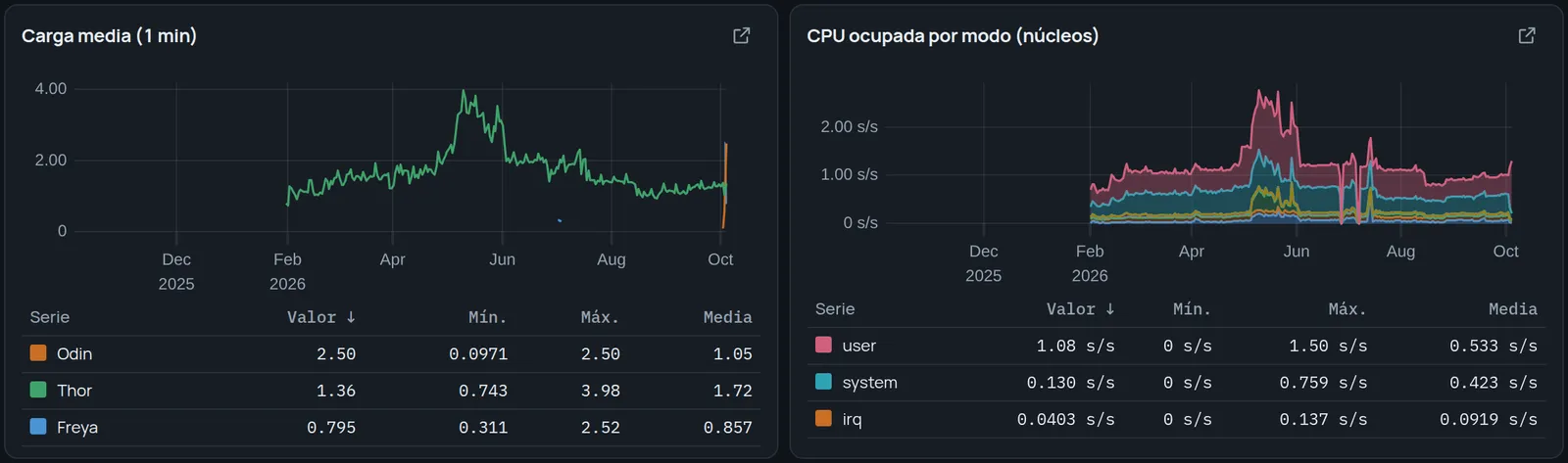
• The 452 queries of my Grafana dashboards run unchanged through its own PromQL engine, and a year of CPU by mode draws in 0.6 s.
• Open source: two container images and a Docker Compose example that runs the whole thing on one machine.

Why not just put OpenTelemetry in ClickHouse

ClickStack was the obvious path, so I measured it first, with my own data. The OpenTelemetry metrics schema writes every point together with its attribute maps: resource attributes, metric attributes, scope. ClickHouse compresses them well, but they are the same maps on every row of a series, millions of times.

3.47 bytes per point, 2.7 of them repeated maps. Loading 17 million samples into it produced merges of up to 5.7 GiB, took more than 10 minutes and ran out of memory three times. The same samples in Atalaya’s schema: 14 seconds and about 250 MB.

Cloud Monitoring’s model, in four tables

Cloud Monitoring, and Monarch, the system behind it, describe a metric once, a time series once, and then only store points. Atalaya does the same:

• Metric descriptors: one row per metric, with its kind (gauge, cumulative, delta or distribution), unit and description.
• Series: one row per time series, identified by a 64-bit hash (xxh3) of its metric and labels. The labels live here, once.
• Points: series, time, value. Nothing else.
• Logs, with the Nomad job, task and allocation of the line.

The collector discovers targets through Nomad, registers each series the first time it sees it, and from then on only sends points. The points table is almost nothing:

CREATE TABLE atalaya.points
(
    Metric   LowCardinality(String),
    SeriesId UInt64,
    Time     DateTime CODEC(DoubleDelta, ZSTD(1)),
    Value    Float64  CODEC(Gorilla, ZSTD(1)),
    Counter  Bool DEFAULT false
)
ENGINE = MergeTree
PARTITION BY toYYYYMM(Time)
ORDER BY (Metric, SeriesId, Time)
TTL Time + INTERVAL 7 DAY;

Sorted by series and then time, DoubleDelta turns regular timestamps into runs of zeros and Gorilla stores each value as the XOR against the previous one. In production the raw table sits at 0.67 bytes per point.

To be fair to VictoriaMetrics: per raw sample it’s more compact, at 0.24 bytes. Atalaya doesn’t win on compression. It wins by not keeping every sample forever.

Coarser as it ages, written at insert time

Every insert into points also feeds two materialized views, which aggregate into a 1-minute and a 10-minute table. Each row of a tier keeps the minimum, maximum, sum and count of its window, the time of its last sample, and a sketch for percentiles:

CREATE MATERIALIZED VIEW atalaya.points_10m_mv TO atalaya.points_10m AS
SELECT Metric, SeriesId, toStartOfInterval(T0, INTERVAL 10 MINUTE) AS Time,
       min(Value) AS Min, max(Value) AS Max, sum(Value) AS Sum, count() AS Count,
       max(T0) AS LastTime,
       quantilesDDStateIf(0.01, 0.5, 0.95, 0.99)(Value, NOT Counter) AS Sketch
FROM (SELECT Metric, SeriesId, Time AS T0, Value, Counter FROM atalaya.points)
GROUP BY Metric, SeriesId, Time;

ClickHouse can also roll rows up when they expire, with TTL … GROUP BY. I tried it and dropped it: it aggregates during merges, holding the groups in memory, and on a homelab box that was the memory-hungry option. The views cost a little extra on every write and never surprise you.

Two details matter more than they look:

• Counters keep their maximum, not their average. A rate over a tier comes from the maximum of each window, and LastTime says when that maximum was read, so a half-filled window (a restart, a gap) doesn’t turn into a spike.
• Prometheus histograms are distributions. Their cumulative buckets are stored as they come; the percentiles of any window come from the difference between the buckets at its end and at its start, in any tier.

Percentiles that survive downsampling

The classic downsampling mistake is keeping each window’s p99 and averaging them later. A day’s p99 is not the average of 144 ten-minute p99s, and the error is largest exactly when something happened.

A sketch can be merged instead. DDSketch places values in logarithmic buckets with a bounded relative error (1 % here, the first parameter of quantilesDD), and 144 ten-minute sketches merge into the sketch of the day. Measured: a daily p99 computed from the 10-minute sketches was 0.7 % off the exact p99 over the raw points. That’s what lets the 10-minute tier live forever and still give the right p99 for any day, months later.

Logs, forever

CREATE TABLE atalaya.logs
(
    Time       DateTime64(3) CODEC(Delta(8), ZSTD(1)),
    Service    LowCardinality(String),
    Host       LowCardinality(String),
    Stream     LowCardinality(String),
    Level      LowCardinality(String),
    Body       String CODEC(ZSTD(3)),
    Resource   Map(LowCardinality(String), String) CODEC(ZSTD(1)),
    Attributes Map(LowCardinality(String), String) CODEC(ZSTD(1)),
    INDEX idx_body lower(Body) TYPE text(tokenizer = 'splitByNonAlpha'),
    INDEX idx_level Level TYPE set(16) GRANULARITY 4
)
ENGINE = MergeTree
PARTITION BY toYYYYMM(Time)
ORDER BY (Service, Time);

No TTL, and monthly partitions so their number stays small over the years. ClickHouse’s text index makes a word search skip whole blocks instead of scanning them. 36 bytes per line, index included.

Moving the log history was the urgent part: VictoriaLogs kept four weeks, and by the time the import ran it had already dropped everything before September 5. The 1.32 million lines that were left now don’t expire.

Bringing eight months of history along

VictoriaMetrics held 36.6 billion samples since February, in 8.3 GiB. Re-inserting them raw would have been pointless, since raw points only live a week. The import goes through Null tables instead: ClickHouse stores nothing in them, and their materialized views write straight into the tiers. Data from the last six weeks lands in both tiers; anything older goes only to the 10-minute one.

ClickHouse itself does the reading: its url() table function pulls each day from VictoriaMetrics’s export API, so the samples never pass through a script. Four workers, one day at a time, took about 12 hours. The import skipped the metrics of the tools being retired, about 10,000 of 23,000 series, because nobody needs Grafana’s own history after Grafana is gone.

One bug nobody warns you about happened right there: retiring Grafana in the middle of the import cut one of the workers. The VictoriaMetrics firewall had a rule for Grafana’s service; when the service disappeared, the firewall sidecar restarted and dropped the connection of the worker that was halfway through June 29. Deleting that day’s partial rows and relaunching the worker from that day fixed it. The other three never noticed.

Where the bytes are, per row:

Table	What a row holds	Bytes per row
points	one sample, 7 days	0.67
points_1m	a minute: min, max, sum, count, sketch	3.5
points_10m	ten minutes, the same fields	7.4
logs	one line, with its text index	36

4.5 GiB on disk for everything, about 23 times less than the same data uncompressed.

It speaks PromQL, so the dashboards came along

Atalaya’s own explorer works like Cloud Monitoring’s: aligners and reducers, queries A, B and C with formulas, comparison against an earlier period. But my eight Grafana dashboards were written in PromQL, so Atalaya also implements the Prometheus HTTP API with its own PromQL engine in Rust, evaluated over the tiers.

The 452 queries of those dashboards run without errors. Against VictoriaMetrics, gauges and irate come out identical. rate differs by up to 12 % over 5-minute windows and 2 % over an hour, because the two engines extrapolate the edges of the window differently.

Another bug nobody warns you about: after the migration, the “CPU Busy” gauge read 21–55 % with the machine at 3 %. The collector flushes every 30 seconds and the dashboard asked for data up to “now”, so the last 60-second window held two samples and the rate was extrapolated from half a window. Prometheus has the same problem; the fix is Grafana’s: relative ranges end 45 seconds in the past. The gauge now reads 3.5 %.

Making it fast: 94 % was reading

Before tuning anything, I measured inside the server. Of a typical dashboard query’s time, 94 % was reading samples from ClickHouse; evaluating the PromQL took 0–3 ms. And ClickHouse was reading 27 to 67 times more rows than it returned: its index works in blocks of 8,192 rows, and one series has about 1,440 points a day, so every series dragged in nearly a whole block.

Three changes:

• Downsample inside ClickHouse, to the step of the chart, as Cloud Monitoring does with its alignment period. A year-long chart draws a few hundred points per series; it doesn’t need the 52,000 ten-minute rows each series has in a year.
• Smaller index blocks, 512 to 2,048 rows instead of 8,192. It can’t be changed in place, so each table was rebuilt and swapped atomically. A one-hour query went from reading 84,806 rows to 21,504.
• Less on the wire: RowBinary instead of TSV between ClickHouse and the server, compressed responses (the metric list went from 465 to 47 KB, an hour of logs from 228 to 9 KB) and panels batched into a single request instead of one each.

Downsampling did the most for long ranges: a year of CPU by mode went from 5.5 to 0.6 seconds, with the server under 100 MB. The full Node Exporter dashboard, 276 queries, now loads in 2.9 seconds with a median of 30 ms per query; VictoriaMetrics answered the same kind of query in about 20 ms inside its own server, so they’re in the same league. The full dashboard set, mostly short ranges, improved less with the rest, 23 %, and the smaller index blocks helped less than I expected: the real weight was in tier rows not yet merged. Every 30-second flush writes its own partial row for the same minute, two per minute, until ClickHouse merges them, and until then a query has to read and combine both.

What it costs to run

The collector is the cheap part: 20–30 MB of memory and 0.1–0.17 % of a core on each node, with its biggest scrape at 150 ms. It spools to disk when ClickHouse is away and survived a ClickHouse restart without losing a batch.

The expensive part was a setting. With 10-second batches, every flush created a part in each table and tier: about 90 new parts a minute for ClickHouse to merge. Going to 30-second batches, flushing ClickHouse’s own system logs once a minute instead of every 7.5 seconds, and sizing reservations to real use left Atalaya reserving 1,020 MHz of CPU against 1,690 for the old stack.

Against what it replaced, measured over one clean hour:

• Disk, memory and reservations are all lower: half the disk, 29 % less resident memory (most of it ClickHouse’s cache) and less than half the memory reserved in Nomad.
• It ingests less, too: 791 points per second against 1,880 samples, because the old stack scraped every 10 seconds and also scraped itself.
• Disk writes are where the old stack wins: 34 KB/s against ClickHouse’s 171. ClickHouse feeds two extra tiers and merges parts; the batch change had already brought it down from 545 KB/s, with 58 % fewer parts and 70 % fewer merges. On an NVMe drive it doesn’t matter.

One write cost an hour can miss: to drop expired rows, ClickHouse rewrites the monthly partition, every 4 hours by default. Across the four tables with a TTL that came to 33 GiB of writes a day. Once a day is enough (merge_with_ttl_timeout = 86400); expired data just stays up to a day longer.

The interface is the structure, not the palette

The first interface copied Cloud Monitoring, and it worked. When I asked for something more attractive, the first round of designs came back as six directions that were one design in six palettes: the same sidebar, the same row of KPI tiles, the same grid of chart cards. A UI is defined by its skeleton; changing the colours on top doesn’t make it a different design.

The second round varied the structure, and each direction turned out to answer a different question:

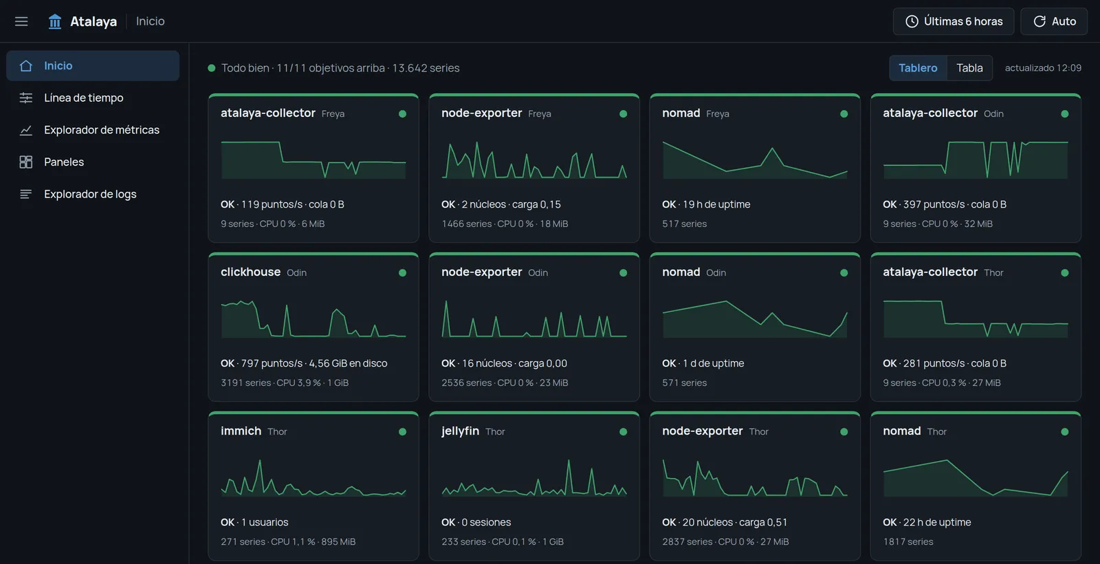
• How is everything right now? A status board with one tile per service, a dense table with one row per host and service, and a map of the homelab.
• What happened? A timeline: one time axis and lanes below it for deploys and restarts, log bursts per service, alerts and a few key metrics.
• Why? A notebook, where an investigation is text, queries and charts in cells.

So they’re one product, not six alternatives. The board and the table are the home, two densities of the same “now”; the timeline is where an investigation starts, and the notebook is where it gets written down.

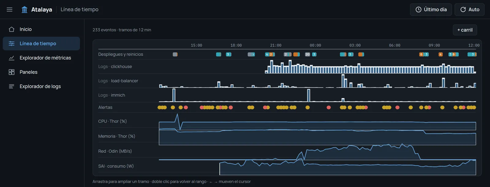
The timeline reads its events from Nomad and the logs, and groups them: a deploy of the collector to the three nodes shows as two events, “3 new allocations” and “3 stopped”, not one per line. Grouping took a day’s worth from 371 events to 220.

What I’d keep from this

• Measure the schema with your data before adopting one. The OpenTelemetry schema is a fine interchange format; as a storage format for metrics it cost 4.6× more per point.
• Downsample at insert time and keep sketches, not percentiles. Averages of p99s lie; merged sketches don’t.
• Find out where the time goes before tuning. The PromQL engine was the tempting target, and it was 0–3 ms of every query.
• In ClickHouse, batch size is a cost. Every insert is a part, every part is a merge.
• If you don’t need “forever”, VictoriaMetrics is hard to beat. Smaller per raw sample, fewer disk writes, and you don’t have to write it.

Try it

Atalaya is on GitHub under the Apache 2.0 license: github.com/mariojcr/atalaya. Each release publishes two images, ghcr.io/mariojcr/atalaya-server and ghcr.io/mariojcr/atalaya-collector, and the repository has a Docker Compose example that runs ClickHouse, the schema, the server, a collector and node-exporter on one machine, with example dashboards and alert rules:

git clone https://github.com/mariojcr/atalaya
cd atalaya/examples/compose
for u in ADMIN READER COLLECTOR; do echo "CLICKHOUSE_${u}_PASSWORD=$(openssl rand -hex 16)"; done > .env
docker compose up -d

The UI is then at http://localhost:8080. Nomad isn’t required: without it, the collector scrapes static targets and reads Docker’s logs. It also reads the host’s hardware (temperatures, fans, CPU energy, GPU, SMART disk health), and the server evaluates alert rules with silences and sends them to ntfy, Telegram or a webhook. The repository has an example for a Nomad cluster as well.

It’s version 0.1.0 and runs my homelab every day. The PromQL engine covers what dashboards commonly use, not the whole language, and sign-in (OpenID Connect) is optional, so without it keep the server on a private network or behind an authenticating proxy.

Still to come: the map of the homelab, and a metric catalog. The collector’s rules can already keep, drop and aggregate metrics per service; applying a catalog that keeps only what the dashboards and alerts use would cut 13,844 series to about 1,400. Bug reports and pull requests are welcome.